第6回 分散分析（第7章） Analysis of Variance

Presentation on theme: "第6回 分散分析（第7章） Analysis of Variance"— Presentation transcript:

1 第6回 分散分析（第7章） Analysis of Variance
回帰モデルにおける分散分析 回帰式の全体的な適合度（分散分析） 平方和の分解 Decomposition of Sum of Squares 全体の散らばり＝説明できた部分＋残差 対応のないデータと，対応のあるデータ 個人（個体）による違いを考える

2 帰無仮説と対立仮説 Null Hypothesis and Alternate Hypothesis
A person has headache （pain in head) Before it, he drank a glass of bad wine. Alternate Hypothesis: what is susceptive; The wine was the cause of the pain. (guilty) Null Hypothesis: Opposite to that hypothesis; The wine was not the cause of the pain. (innocent)

3 棄却と採択 Rejection of the Null Hypothesis
When we permit the Null Hypothesis, the probability of the realized event is calculated. Calculate the probability of headache when he did not drink such a wine. If the probability is too small (smaller than your critical probability), you can reject the null-hypothesis and approve the alternate hypothesis. The wine was the cause of the pain. (guilty) If the probability is not too small, you cannot say anything. (not actively approve the null hypothesis). The wine was not the cause of the pain. (innocent)

4 連続変数と棄却域 Critical Value for Continuous Variable
We take a continuous variable such as headache duration, we can set the critical region, more easily, based on the usual probability density. If he had headache with certain large probability, when drinking no wine, we cannot reject the Null Hypothesis. Probability Density under the Null Hypothesis 0.05 No-ache 60min Ache Duration of headache 4

5 F分布 （F distribution) 確率密度関数 自由度(f1,f2) のF 分布 F分布もχ2分布と関係がある。
X, Y が独立でそれぞれ自由度f1, f2 のχ2 分布に従うとき、 は自由度(f1, f2) のF 分布に従う。 したがって2 つの標本群から計算した分散の比をとると、その統計量はF 分布に従う．

6 　F分布表　（F distribution)

7 Regressed Sum of Squared
目的変数をどの程度[記述]出来たか？ なる説明式がある場合 Xiによる説明式がない場合 回帰（Xiで説明 できた　y　から のずれ） yiの推計値 として、 平均値 y を 使うしかない Y Y 残差･誤差 X 回帰平方和 Regressed Sum of Squared 平均値周りの バラツキ（全平方和） Total Sum of Squares 決定係数 説明できた 平方和の割合 残差平方和 Error Sum of Squared

8 平方和（散らばり）の分解 Decomposition of Sum of Squared
全体の散らばり（Total)を分解 　説明できた散らばり（Regressed) 　　　＋残りの散らばり（Error) それぞれを平方和（Sum of Squared)で評価　ST=SR+SE 帰無仮説：SRとSEは統計的に同程度のもの そのときには、Fo＝VR/VEはF分布(自由度fR, fE)に従う 　　　　　　　ただしVR=SR/fR， VE=SE/fE

9 回帰による記述（説明）力の検定 回帰平方和が統計的に大きな意味を持っているか？ 分散分析表を作り、F検定を行って判断する。
帰無仮説：回帰平方和は誤差平方和と同程度の大きさ 　（回帰式は、誤差に比べて大きな説明力はない） 対立仮説：回帰平方和は誤差平方和より大きい 　（回帰式によって誤差よりもかなり大きい部分が説明できた）

10 回帰による記述（説明）力の検定例 帰無仮説：回帰平方和は誤差平方和と同程度の大きさ （回帰式は、誤差に比べて大きな説明力はない）→棄却
　（回帰式は、誤差に比べて大きな説明力はない）→棄却 対立仮説：回帰平方和は誤差平方和より大きい 　（回帰式により、誤差よりもかなり大きい部分が説明できた） Multiple R-squared: , Adjusted R-squared: F-statistic: on 2 and 6 DF, p-value:

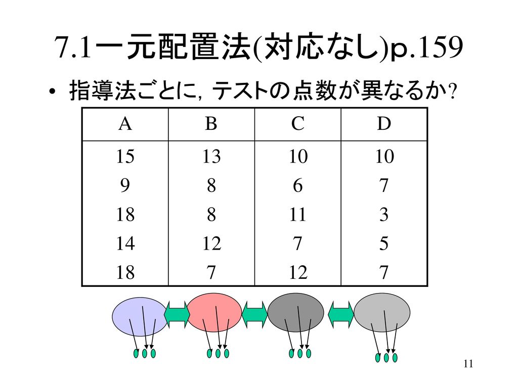
11 7.1一元配置法(対応なし)ｐ.159 指導法ごとに，テストの点数が異なるか? A B C D 15 9 18 14 13 8 12 7
10 6 11 3 5

12 変動の分解 ＝ ＋ 観測値 全体平均 全体変動 ＝ ＋ 全体変動 群間平均 群内変動(残差) A B C D 15 9 18 14 13 8
12 7 10 6 11 3 5 A B C D 10 A B C D +5 -1 +8 +4 +3 -2 +2 -3 -4 +1 -7 -5 ＝ ＋ 観測値 全体平均 全体変動 A B C D +5 -1 +8 +4 +3 -2 +2 -3 -4 +1 -7 -5 A B C D 4.8 -0.4 -0.8 -3.6 A B C D 0.2 -5.8 3.2 -0.8 3.4 -1.6 2.4 -2.6 0.8 -3.2 1.8 -2.2 2.8 3.6 0.6 -3.4 -1.4 -0.6 ＝ ＋ 全体変動 群間平均 群内変動(残差)

13 平方和の評価 ＝ ＋ 全体変動 群間平均 群内変動(残差) 平方和 322 平方和 184 平方和 138 分散16.94＝322/19
A B C D +5 -1 +8 +4 +3 -2 +2 -3 -4 +1 -7 -5 A B C D 4.8 -0.4 -0.8 -3.6 A B C D 0.2 -5.8 3.2 -0.8 3.4 -1.6 2.4 -2.6 0.8 -3.2 1.8 -2.2 2.8 3.6 0.6 -3.4 -1.4 -0.6 ＝ ＋ 全体変動 群間平均 群内変動(残差) 平方和　322 平方和　184 平方和　138 分散16.94＝322/19 分散 /3 分散8.6=138/16 自由度19＝20-1 自由度3＝4-1 自由度16=4(5-1) 13 F=61.33/8.625=7.11

14 F分布表 （F distribution) 7.11 3.24 Under the null-hypothesis,
The Ratio of Variance goes beyond the observed value (7.111) with Probability smaller than 0.05. You can reject the null-hypothesis: The inter-group variation is statistically different from the inner-group. 14 7.111＞F(0.05:3,16)＝3.24 14

15 Rによる計算 aov() > 統計テスト2
[1] > 指導法2 [1] A A A A A B B B B B C C C C C D D D D D Levels: A B C D > oneway.test(統計テスト2~指導法2,var.equal=TRUE) One-way analysis of means data: 統計テスト2 and 指導法2 F = , num df = 3, denom df = 16, p-value = > summary(aov(統計テスト2~指導法2)) Df Sum Sq Mean Sq F value Pr(>F) 指導法 ** Residuals --- Signif. codes: 0 ‘***’ ‘**’ 0.01 ‘*’ 0.05 ‘.’ 0.1 ‘ ’ 1 >

16 7.2一元配置法(対応あり)ｐ.175 3科目に対する好意度の評価 学生 田中 岸 大引 吉川 荻野 7 8 9 5 6 4 1 3 2
線形代数 微分積分 確率統計 田中 岸 大引 吉川 荻野 7 8 9 5 6 4 1 3 2 16 16

17 変動の分解 ＝ ＋ 観測値 全体平均 全体変動 全体変動 ＝ ＋ ＋ 条件(科目間) 個人差(個人間) (残差) 線 微 確 田 岸 大 吉
荻 7 8 9 5 6 4 1 3 2 線 微 確 田 岸 大 吉 荻 5.53 線 微 確 田 岸 大 吉 荻 1.46 2.46 3.46 -0.53 0.46 -1.53 -4.53 -2.53 -3.53 ＝ ＋ 観測値 全体平均 全体変動 線 微 確 田 岸 大 吉 荻 1.46 -1.53 0.06 線 微 確 田 岸 大 吉 荻 1.13 0.46 2.13 -2.86 -0.86 線 微 確 田 岸 大 吉 荻 -1.13 0.53 -0.13 0.86 -0.46 1.26 -0.06 -0.73 -0.26 全体変動 ＝ ＋ ＋ 17 条件(科目間) 個人差(個人間) (残差)

18 平方和の評価 ＝ ＋ ＋ 全体変動 条件(科目間) 個人差(個人間) (残差) 平方和 22.53 平方和 6.133 平方和 45.06
線 微 確 田 岸 大 吉 荻 1.46 -1.53 0.06 線 微 確 田 岸 大 吉 荻 1.13 0.46 2.13 -2.86 -0.86 線 微 確 田 岸 大 吉 荻 -1.13 0.53 -0.13 0.86 -0.46 1.26 -0.06 -0.73 -0.26 ＝ ＋ ＋ 全体変動 条件(科目間) 個人差(個人間) (残差) 平方和　22.53 平方和　6.133 平方和　45.06 平方和　73.73 分散11.267 分散　0.767 分散11.267 自由度 14＝15-1 自由度2＝3-1 自由度4＝5-1 自由度8=4(3-1) Fo=11.267/0.767=14.69>F(2,8,0.05)=4.64 18 Fo=11.267/0.767=14.69>F(4,8,0.05)=3.84

19 Rによる計算 aov() > 好意度 [1] 7 8 9 5 6 5 4 7 1 3 8 6 7 2 5 > 科目
[1] 線形代数 線形代数 線形代数 線形代数 線形代数 微分積分 微分積分 微分積分 微分積分 [10] 微分積分 確率統計 確率統計 確率統計 確率統計 確率統計 Levels: 確率統計 線形代数 微分積分 > 人 [1] 田中 岸 大引 吉川 荻野 田中 岸 大引 吉川 荻野 田中 岸 大引 吉川 荻野 Levels: 荻野 岸 吉川 大引 田中 > summary(aov(好意度~科目)) Df Sum Sq Mean Sq F value Pr(>F) 科目 Residuals

20 Rによる計算 aov() > summary(aov(好意度~人))
Df Sum Sq Mean Sq F value Pr(>F) 人 * Residuals --- Signif. codes: 0 ‘***’ ‘**’ 0.01 ‘*’ 0.05 ‘.’ 0.1 ‘ ’ 1 > summary(aov(好意度~科目+人) ) Df Sum Sq Mean Sq F value Pr(>F) 科目 ** 人 *** Residuals